Liberty Instruments, Inc.

The Waterfall Plot: What it means and how it is generated

(reprinted from Speaker Builder Magazine)

The Waterfall plot in Liberty Audiosuite or IMP is more properly known as the "Cumulative Spectral Decay" (CSD) plot. This plot technique is generally credited to Fincham and Bernam (of KEF) who used it to detect resonances and internal box reflections in loudspeakers.

A waterfall is a presentation of both frequency domain and time domain data on a single graph. Time domain data is voltage or pressure as a function of time, usually in the form of a measured impulse response (origination from a pulse or MLS measurement), which covers all time (but can be assumed to decay to insignificant levels within a finite time). The frequency domain version is the decomposition of the time domain impulse response into periodic cosine waveforms via Fourier analysis (the impulse response can be represented as a summation of an infinite number of cosine waves of different frequencies). In any combined time-frequency analysis, there are inherent resolution limitations due to the related (reciprocal) relationship of time (seconds) and frequency (per second). One cannot, for instance, talk about a frequency at a point in time -- it is rather meaningless to discuss a periodic wave unless (at the very least) the time length of that period is considered. Hence, a frequency component cannot be said to start or stop at a specific time. But a band of frequencies can be analyzed in terms of its energy within a said time segment.

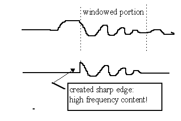
One relatively obvious way to do this is to select (or "window") only a portion of a time signal and perform a Fourier analysis over that section only, as if the time signal were zero elsewhere. This does generate some problems in that extraneous frequency components can be erroneously created by suddenly chopping a non-zero section of a signal to zero at the edges of the window. Use of windows which are tapered, on both edges of the time segment or on only one, can help to reduce (but not eliminate) this effect.

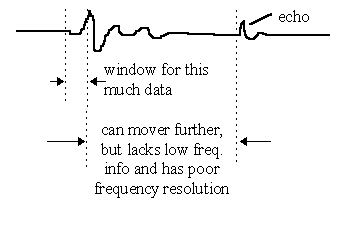
If the time length of the segment is kept constant, but its position in the time continuum is varied as one axis of the plot and the resulting spectrum of the Fourier analysis is shown versus the remaining axes, a plot known as the Short-Term Fourier Spectrogram results. This plot is an attempt to show "frequency response versus time". It has the disadvantage that it can contain no valid information for frequencies below 1/(time segment length); therefore, to get data down to 500Hz, the segment length must be at least 2msec long. If, however, an echo occurs from a realworld measurement at 3msec after the beginning of the impulse response, the time segment can be swept over only 1msec if the echo characteristic is not to be included; this wouldn’t give much of a span for the time axis. If shorter time spans are analyzed, a frequency-vs-time plot can be made over a longer time length, but can only show data for very high frequencies and at poor resolution.

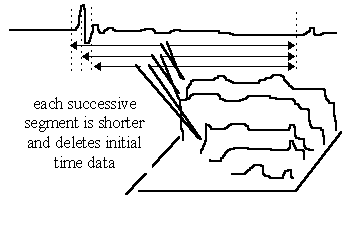
If, on the other hand, the entire active time trace is included for the initial transformation and then the position of the later edge of the window is held fixed relative to the beginning point of the impulse response, and only the earlier edge is varied, a CSD or LAUD waterfall plot results. Because the length of each time segment is being shortened with each successive step in the "time sweep", the lowest resolvable frequency increases (loses resolution) at later points in the plot. At the first traces of the plot, frequencies down to the anechoic limit can be displayed; successive curves will be valid to approximately 1/( windowed time span). In IMP and Audiosuite (and PRAXIS), data below the LF resolution cutoff are not plotted, resulting in an easily identified drop edge on the later traces of the plot; some other packages plot such below-resolution LF data anyway, although it is not meaningful and can lead to incorrect conclusions based on information which simply isn’t there.

The CSD waterfall does NOT show frequency response versus time! It shows that (approximate) frequency content contribution to a total response which occurs after the (relative) time shown in the time axis. At t=0 on the CSD plot, the entire frequency response is drawn, as the total response occurs after this time. At t=1msec the CSD plot shows the contribution to the frequency response which occurs after 1 msec but not before 1msec, and so on. But note the caution previously stated above: frequencies cannot start at a precise time! -- CSDs often show the user’s technique more than the speaker’s quality! Also note that if an echo pulse is included in the time segment selected for the waterfall plot, the frequency contribution of the echo will be present in the plot for all times before the echo occurs.

CSD waterfalls are most often used to detect and display resonant behavior in speaker cones, boxes or horns. A resonance will show up as a long decaying ridge along the time axis, due to the "ringing" of the resonance over time. The data shown is VERY SUSCEPTIBLE to measurement and display conditions. The inherent windowing operation is hacking into the most active part of the impulse response, the result of which will change depending on the window shape used, on the step size being used for the waterfall graphing routine, on display scales, on the low-frequency (even below resolution) content and phase, etc. Each curve trace on its own cannot be said to carry much useful information -- it is the overall plot, the ridges, shelves and valleys of the overall surface which are revealing definitely in a qualitative, but in only a slightly quantitative, way.

If one, for whatever reason, wanted to find the waterfall curve value at a point in time and at a specified frequency and read off a dB value for same, he need only recreate the window edge condition for the waterfall plot and perform the corresponding FFT. For example, assume a waterfall plot has been made normally by setting the time markers so that marker number 1 is just before the activity in the time impulse response and marker number two is just before the first significant reflection. You want to read off a value at the waterfall plot’s "1.4 msec" trace, and at 3.3kHz. Merely go back to the time domain plot (by pressing F1). Move marker number 1 to a position 1.4msec to the right of its current position, go to the transform menu and select "FFT". The curve corresponding to the 1.4msec trace of the waterfall plot will result, and you can use the frequency domain markers to read off any values of interest.